Kodeclik Blog
Implementing the quadratic formula in Python
Quadratic equations appear everywhere in mathematics, science, engineering, and even in everyday problem solving. In this blogpost, we’ll review what the quadratic formula is, how to implement it correctly in Python, how to handle special cases like imaginary roots, and some common pitfalls to avoid. We’ll also look at a real-world application and demonstrate how libraries like NumPy can handle the computation for you.
Table of Contents
What is the quadratic formula?
When the leading coefficient is zero
How the discriminant affects the solutions
The quadratic formula in Python using math.sqrt()
The quadratic formula in Python using cmath
Using numpy instead of writing your own formula
Common mistake 1: Missing parentheses
Common Mistake 2: Using math.sqrt for negative discriminants
Common Mistake 3: Forgetting to handle the case a=0
Real-world application: Projectile motion
Summary
What is the quadratic formula?
A quadratic equation is an equation of the form:

where a, b, and c are constants, and it is assumed that a is not zero (otherwise it would not be a quadratic equation). In other words, a quadratic equation is one where the highest degree is 2.
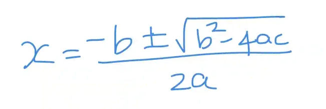
The quadratic formula gives the solutions (also called roots) of this equation:

The expression under the square root is called the discriminant.
When the leading coefficient is zero
If a=0, the equation is no longer quadratic. The equation reduces to:

This is a linear equation. The solution is simply x = -(c/b). So any quadratic formula implementation must check whether a is zero before proceeding.
How the discriminant affects the solutions
Note that the discriminant is the expression inside the square root. Thus, based on whether the discriminant is positive, zero, or negative, we get different possibilities.
If the discriminant is > 0, then we will have two distinct (real) roots. If the discriminant is equal to 0, then we will have one repeated (real) root. If the discriminant is less than 0, then we have two complex (imaginary) roots.
The quadratic formula in Python using math.sqrt()
Here’s a basic Python program to implement the quadratic formula.
import math

def quadratic_roots_real(a, b, c):
    if a == 0:
        return -c / b   # Linear case

    discriminant = b**2 - 4*a*c
    if discriminant < 0:
        raise ValueError("This version only supports real roots.")

    root1 = (-b + math.sqrt(discriminant)) / (2*a)
    root2 = (-b - math.sqrt(discriminant)) / (2*a)
    return root1, root2

# Example usage:
print(quadratic_roots_real(1, -3, 2))
Note that the program first checks if the leading coefficient is zero, in which case it is a linear equation and we can simply give the solution using the linear formula. Also note that we are also checking if the discriminant is less than zero before applying the quadratic formula. The output will be:
(2.0, 1.0)The quadratic formula in Python using cmath
If the discriminant is less than zero, recall that the square root of the discriminant will not a real number. Python’s math.sqrt cannot compute the square root of a negative number, but cmath.sqrt can. So a better approach is to use the cmath module in Python to support complex numbers naturally.
import cmath   # supports complex numbers

def quadratic_roots(a, b, c):
    if a == 0:
        # Not a quadratic equation
        return -c / b

    discriminant = b**2 - 4*a*c
    root1 = (-b + cmath.sqrt(discriminant)) / (2*a)
    root2 = (-b - cmath.sqrt(discriminant)) / (2*a)
    return root1, root2

# Example usage:
print(quadratic_roots(1, -3, 2))    # Two real roots
print(quadratic_roots(1, 2, 1))     # One repeated root
print(quadratic_roots(1, 0, 1))     # Complex roots
If you run this code, you will get:
((2+0j), (1+0j))
((-1+0j), (-1+0j))
(1j, -1j)
Note that all lines represent solutions with both real and imaginary components. The first two lines are for the cases where there are real roots (not repeated and repeated, respectively). You can notice this by the zero component of the imaginary component (denoted by “j”).
Using numpy instead of writing your own formula
If you prefer to avoid implementing the formula, numpy provides a built-in solver:
import numpy as np

coeffs = [1, -3, 2]   # corresponds to x^2 - 3x + 2
roots = np.roots(coeffs)
print(roots)
The output will be:
[2. 1.]Note that np.roots works for polynomials of any degree, not just quadratics.
Common mistake 1: Missing parentheses
Many beginners accidentally write:
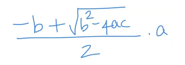
(-b + math.sqrt(b**2 - 4*a*c)) / 2 * aThis will be interpreted as:

which is obviously not the formula. The correct expression is:
(-b + math.sqrt(b**2 - 4*a*c)) / (2*a)Common Mistake 2: Using math.sqrt for negative discriminants
Use cmath.sqrt instead of math.sqrt if complex numbers are possible.
Common Mistake 3: Forgetting to handle the case a=0
If you are implementing the formula yourself instead of using a built-in library, make sure to check for the case when the leading coefficient (i.e., a) is zero. If you do not do this, your program may divide by zero.
Real-world application: Projectile motion
In physics, we encounter problems like:
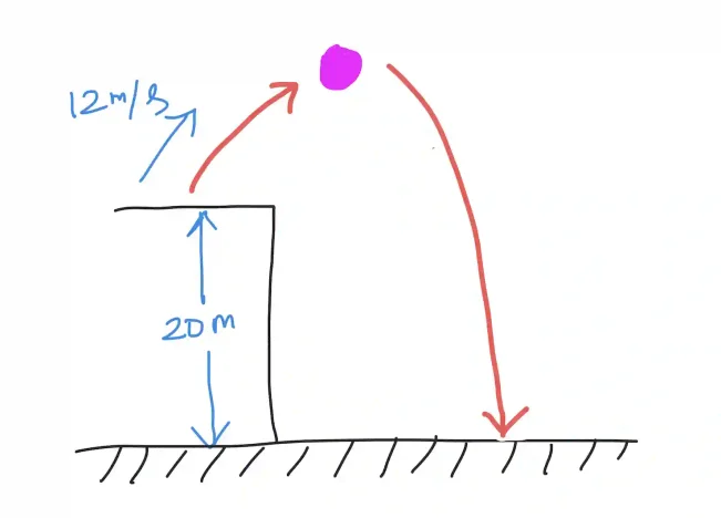
A ball is thrown straight up from a balcony that is 20 m above the ground with an initial speed of 12 m/s. Assuming standard acceleration due to gravity and no air resistance, when does the ball hit the ground?
We can represent this situation as:

To solve this problem, the height (in meters) after t seconds is:

For our problem, this can be cast as:

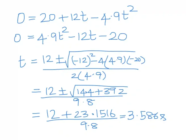
Because we want h(t)=0, the equation can be written and solved as:

We can also use our Python programs above to find that the solution is approximately 3.586 seconds after it is thrown, as calculated above.
Summary
The quadratic formula is a powerful tool for solving equations. In Python, we can implement the formula directly, but we must be careful with parentheses, negative discriminants, and the special case where a=0. Using cmath.sqrt allows us to handle both real and complex roots seamlessly, while numpy’s np.roots function provides an even higher-level solution when working with general polynomials. With these tools, Python makes solving quadratic equations both precise and robust.
Enjoy this blogpost? Want to learn Python with us? Sign up for 1:1 or small group classes.