Kodeclik Blog
Calculating numerical gradients using numpy.gradient()
numpy is a very popular library for data manipulation and scientific computing in Python. One of its many useful features is the ability to calculate numerical gradients of functions using the gradient function. In this post, we'll explore what the gradient function is, how it works, and give examples of how it can be used.
The gradient function in numpy is a method for computing the numerical gradient of a function. The gradient is a vector that points in the direction of the steepest ascent of a function at a given point. It is often used in optimization problems to find the minimum or maximum of a function.
In numpy, the gradient function takes an array of values as input and computes the numerical gradient along a specified axis. The resulting gradient array has the same shape as the input array.
The gradient values can be calculated from the derivative of a function, which is the rate of change of the function at a particular point. However, in practice it is often difficult or impossible to calculate this derivative analytically. Numerical methods like numpy’s gradient function can be used to approximate the derivative of a function at a point by calculating the change in function values over a small interval of h.
Let us suppose we wish to calculate the gradient of the cubic function f(x) = x*x*x. It is well known that the gradient is f’(x) = 3*x*x. Let us see how we can compute this numerically using numpy.gradient().
Consider the following piece of code:
import numpy as np

def f(x):
    return x*x*x

xvalues = np.array([1,2,3])
print(xvalues)

yvalues = f (xvalues)
print(yvalues)

print(np.gradient(yvalues))
In the above code we first define a function that computes the cube of a given number. Then we use this function to map an array of inputs (the xvalues) to an array of outputs (the yvalues). Finally, we pass on yvalues as the argument to the np.gradient() function.
The gradient is computed using second order accurate central differences in the interior points and either first or second order accurate one-sides (forward or backwards) differences at the boundaries. The returned gradient hence has the same shape as the input array.

The output in this case will be:
[1 2 3]
[ 1  8 27]
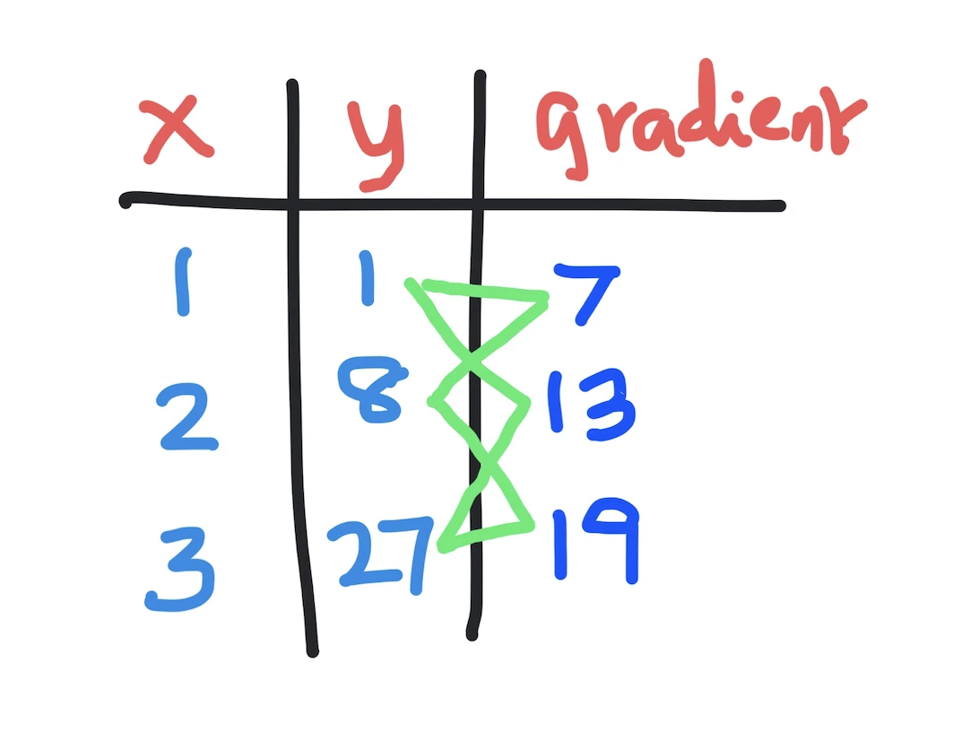
[ 7. 13. 19.]
The first two lines are self-explanatory. For the last line, note that 7 is (8-1)/(2-1). Similarly, 13 is (27-1)/(3-1) and 19 is (27-8)/(3-2). Note that if we were to do this analytically, the derivatives will be given by 3*x*x, or [3 12 27] which is not quite the same as what is returned. This is because numpy.gradient() uses finite difference approximations (as shown by the above calculations) which have approximation errors. Also note that the gradient for x=2 is more accurate than the gradient computed at the end points, as is to be expected.
Note that in the above code, the gradient function takes only one argument (the yvalues). The x-values are actually assumed implicitly. We can pass on explicitly x-values like so;
import numpy as np

def f(x):
    return x*x*x

xvalues = np.array([1,2,3])
print(xvalues)

yvalues = f (xvalues)
print(yvalues)

print(np.gradient(yvalues,[1,2,3]))
This will give the same output as before:
[1 2 3]
[ 1  8 27]
[ 7. 13. 19.]
This format is useful when the x-values are not uniformly spaced (or even if they are uniformly spaced but not starting at 1 as is the case here).
You can also use numpy.gradient() to find the gradients of a 2D field i.e., a function that changes over both x and y directions. In this case for each point there will be two gradients, along each dimension. Here is some Python code for this purpose:
import numpy as np

# Create a two-dimensional array
x = np.array([[1, 2, 3], [4, 5, 6], [7, 8, 9]])

gradient_x, gradient_y = np.gradient(x)

# Print the results
print("Gradients along the x-axis: \n", gradient_x)
print("Gradients along the y-axis: \n", gradient_y)
The output will be:
Gradients along the x-axis:
[[3. 3. 3.]
[3. 3. 3.]
[3. 3. 3.]]
Gradients along the y-axis:
[[1. 1. 1.]
[1. 1. 1.]
[1. 1. 1.]]
as expected. Note that along the x-axis, all ratios of differences amount to 3 (e.g., (4-1)/(2-1)). Along the y-axis, they all amount to 1 (e.g., (5-4)/(5-4)).
So in summary the numpy gradient function calculates the numerical gradient of a given function. The gradient of a function is a vector that points in the direction of the maximum rate of change of the function at a particular point. In other words, it measures how quickly the function changes in different directions.
If you liked learning about numpy.gradient() checkout our blogpost about numpy.split().
Interested in more things Python? Checkout our post on Python queues. Also see our blogpost on Python's enumerate() capability. Also if you like Python+math content, see our blogpost on Magic Squares. Finally, master the Python print function!
Want to learn Python with us? Sign up for 1:1 or small group classes.