How to find the line of best fit in Desmos

Let us learn how to find the line of best fit using Desmos, the graphing calculator!

Step 1: Create some data

Let us create some data! Login to Desmos and click on the “+” (Add Item) option on the top-left corner of your Desmos page. Choose the “Table” option. Enter a set of numbers like so:

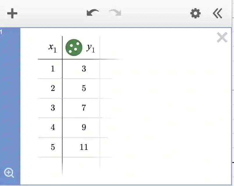
The data for this example could be viewed as coming from a carnival experience. In this example, x could denote the number of rides you take on the carnival and y denotes the price you pay. Note that there is an entrance fee of $1 and each ride costs $2. So to take 5 rides, you need to pay 5*2+1 = 11. This formula explains all the entries of the above table.

Step 2: Create a linear equation

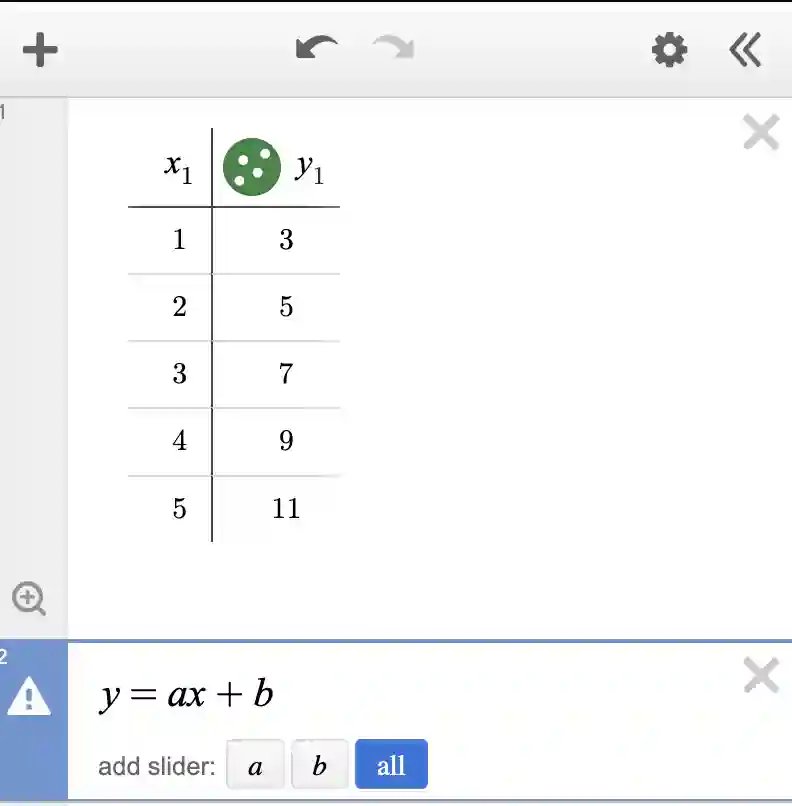
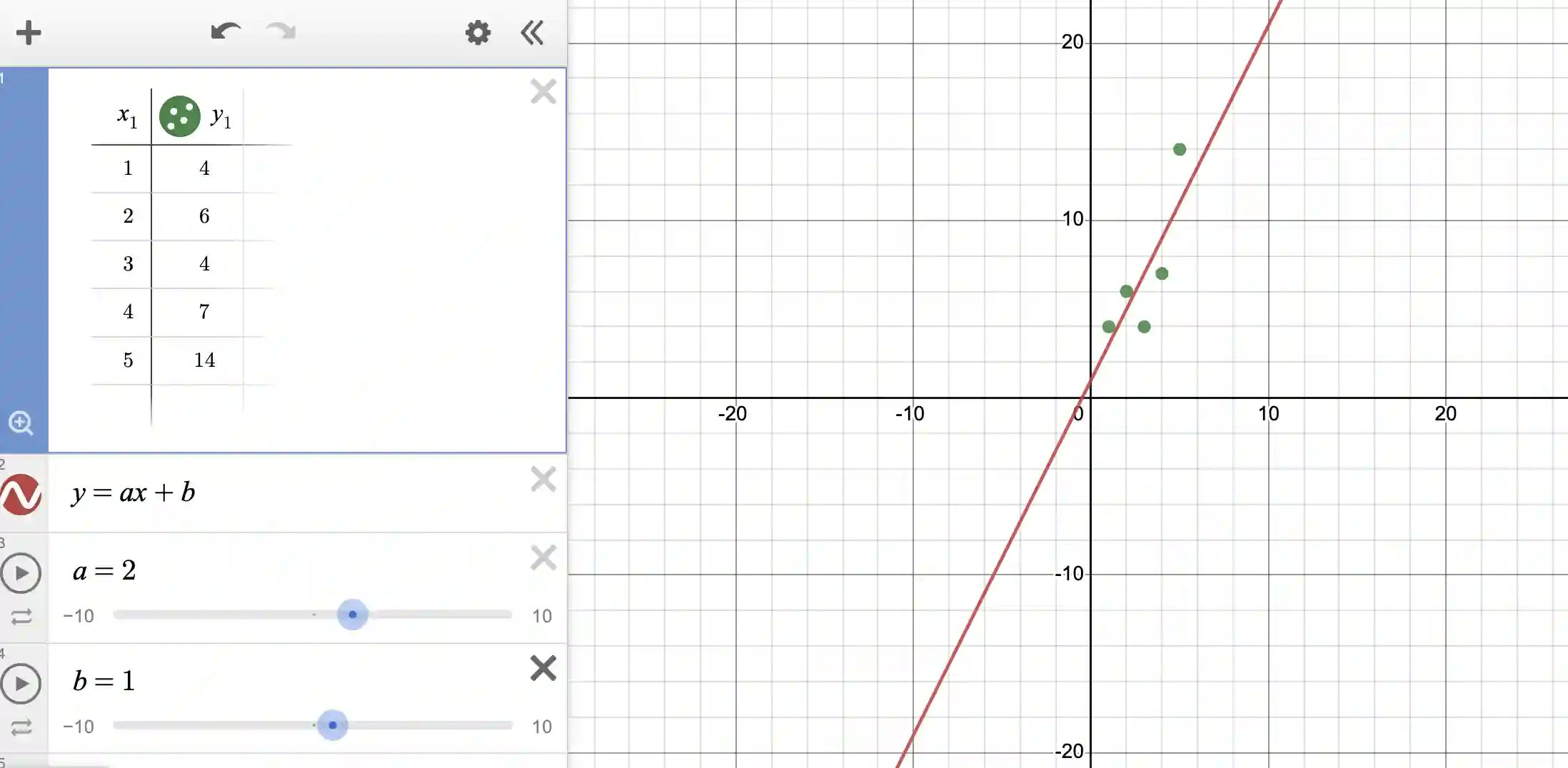
Now let us create a new cell and write “y=ax+b” in it.

Step 3: Add and adjust sliders

Press “all” in the slider options, and voila you will see that your interface has become:

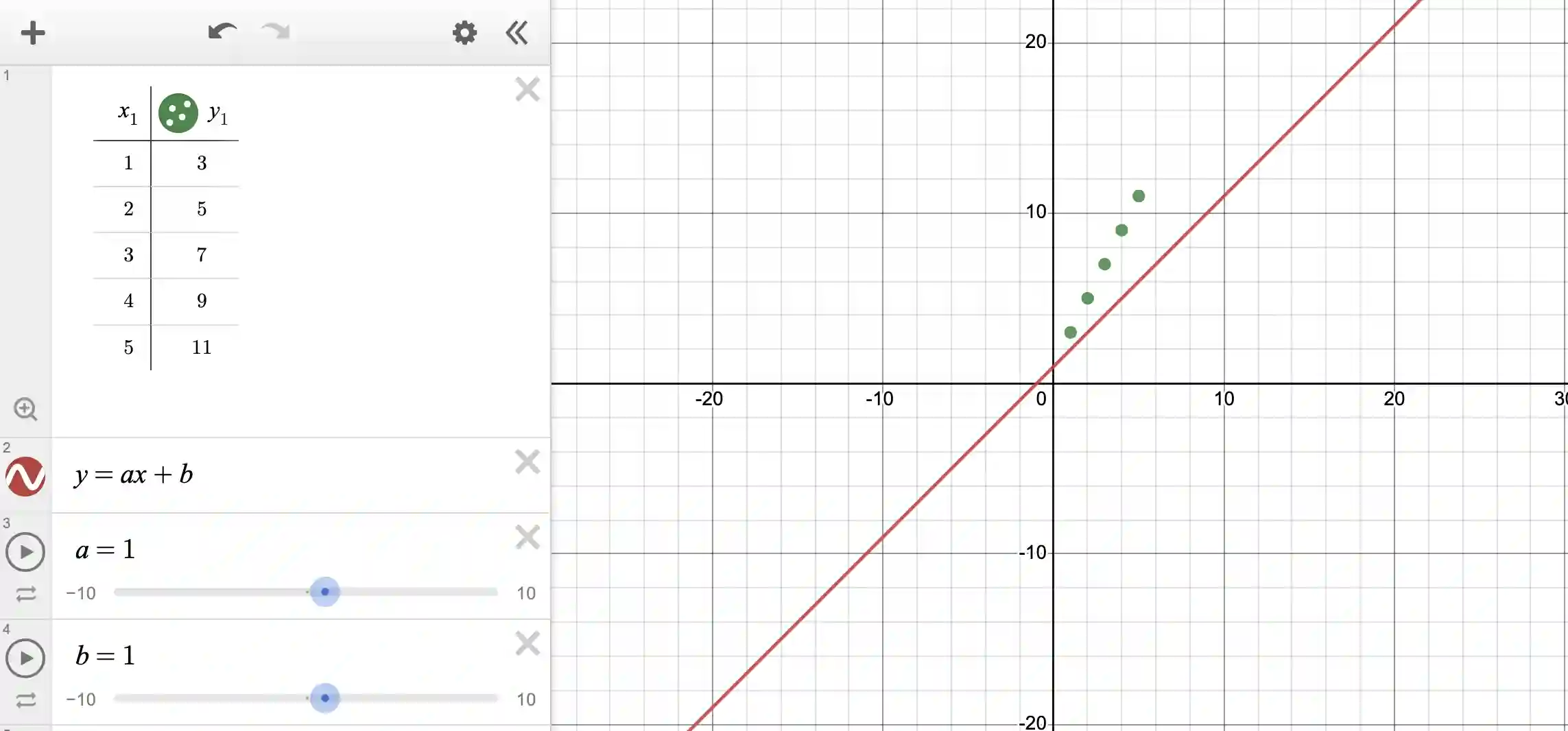
You will see that Desmos has given you sliders for the variables a and b and given both of them default values of 1 (each). It has further plotted the line y=ax+b with these values; in other words y=x+1.

But because you now have sliders, you can move the sliders to try to get a good fit, like so:

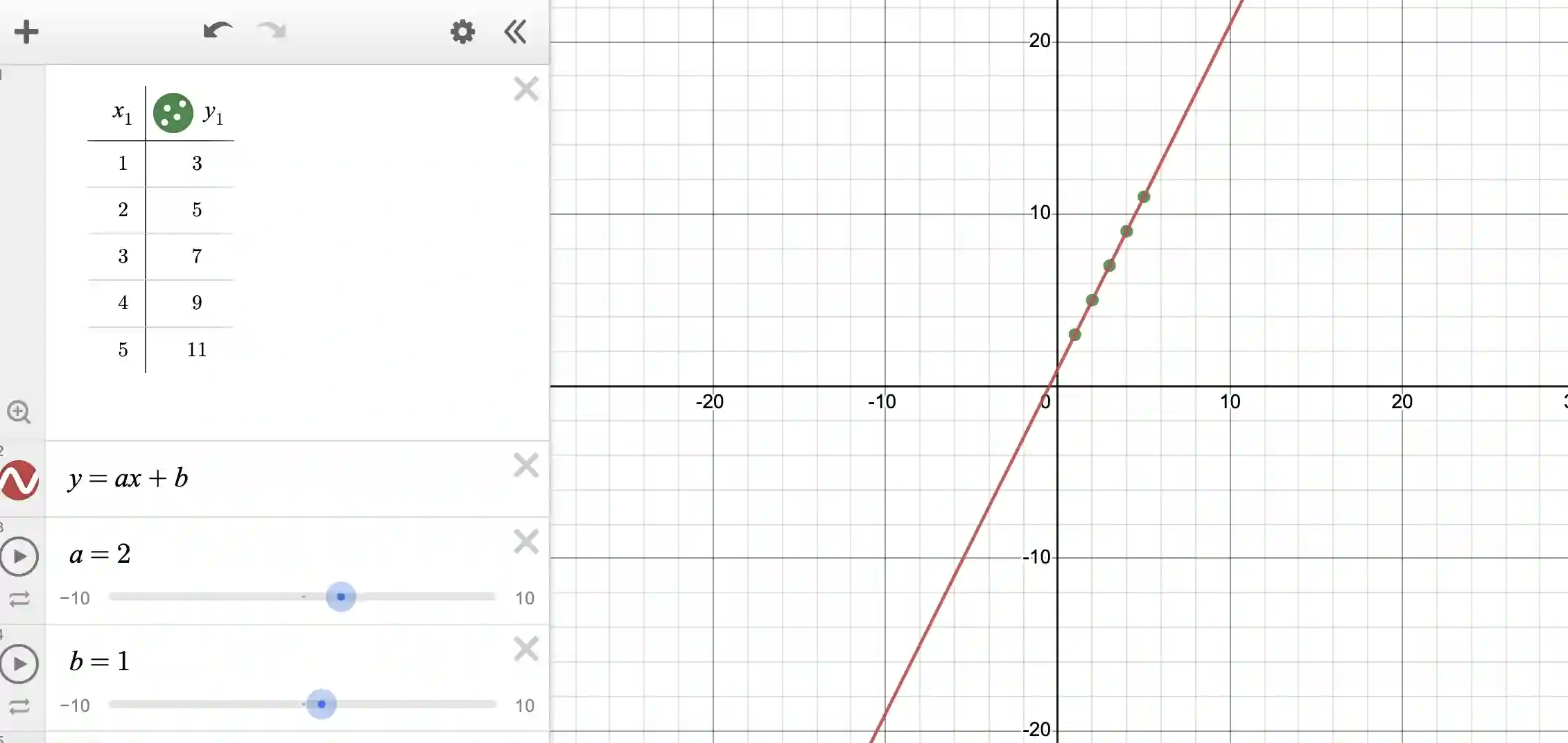
Note that only the slider for “a” needs to be experimented with (because the slider for “b” already started with the correct value of 1).

Step 4: Make data more realistic

Usually in the real world, data is never this nice (ie “well-behaved”). There is usually noise in the data, or other imperfections in measurement. So let us tinker with our data to create some noise:

Note that we have now messed up our data so that the line is no longer a fit. What is more, there will be no line that will be a fit because the data does not follow the rules of linear variation!

What we can do is: even though there is no line that is a fit, we can try to find a line that has the best fit possible. This is called the “line of best fit”.

Step 5: Find the line of best fit

Finding the line of best fit is quite easy in Desmos!

Create a new cell and write y_1 ~ ax_1 + b. Note that we are using the exact column names from our table, namely x_1 and y_1. Further, we are using tilde in place of the equal symbol. If you write this and press enter, you will get:

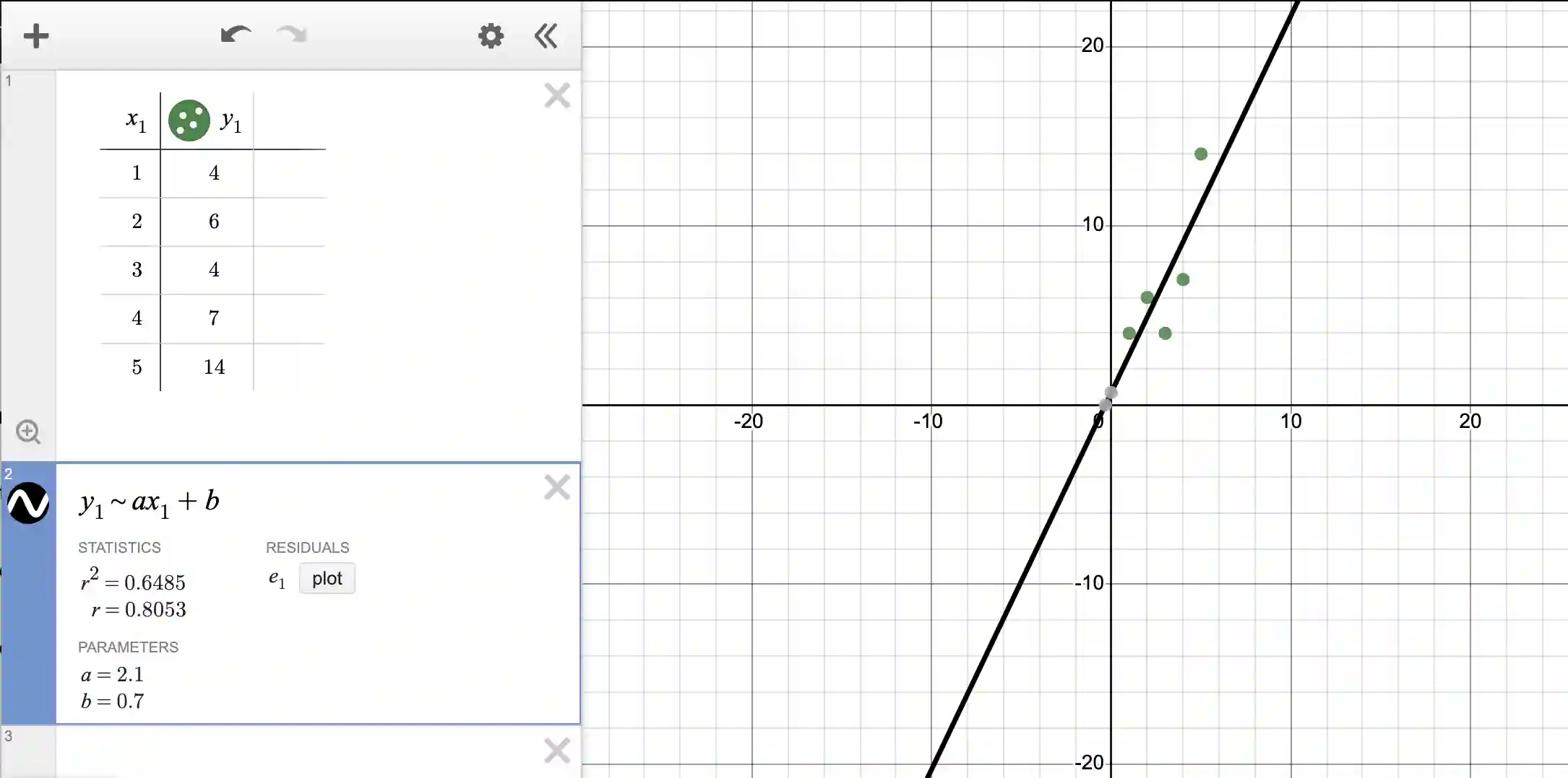
Note that Desmos has calculated for you a best fit line! Note that sometimes the points are really close to the line, sometimes they are not close but are on both sides of the line. In other words, the best fit line “goes through” the points to reduce the errors as much as possible. It is not possible to reduce the error to zero since the points do not lie on a line!

Next, you can notice that the (best fit) line’s coordinates are given by y=2.1x + 0.7. It is interesting that this is really close to our ideal line (from Step 3) of y=2x+1. This is not surprising because we started with data from that equation and then fudged the values.

Step 6: Analyze errors

Next, note that you have an r^2 value. This is the coefficient of determination, a number that tells us how well the regression line fits the data. It's like a measure of how much the independent variable (the “x” in our case) explains the variation in the dependent variable (the one we want to predict, or our “y”). The value of r^2 is always between 0 and 1. If it's close to 1, it means that the independent variable does a good job of predicting the dependent variable. If it's close to 0, it means it's not doing a good job. So, the closer it is to 1, the better the regression line fits the data.

In our case, because r^2 is 0.6485, it means 64.85% of the variation is explained by our model.

To understand how this number was arrived at, press the “plot” button next to the residuals. This will update the plot as:

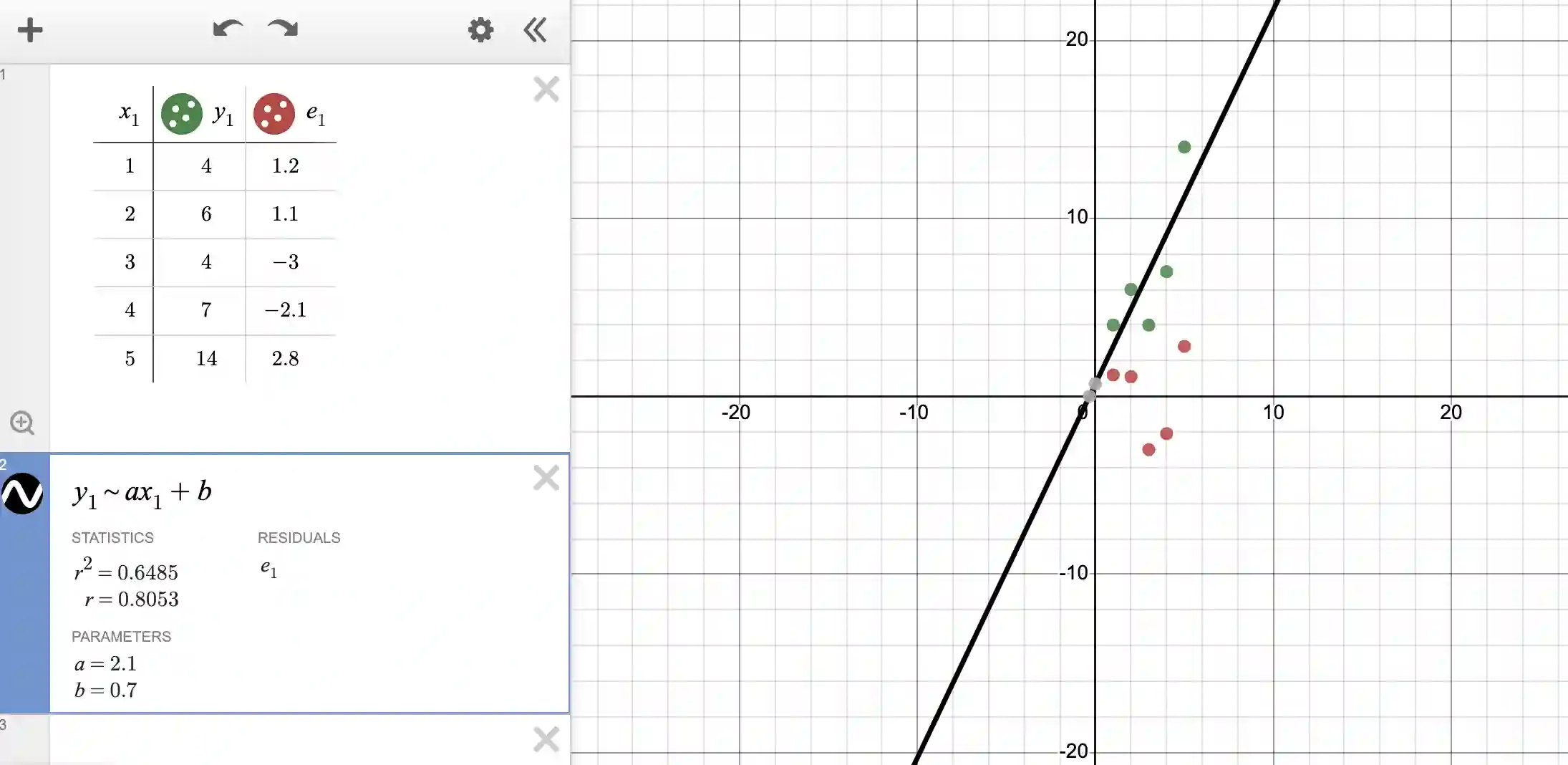
Observe that both the table and the graph have been updated. Note that the error in each value is now recorded next to the table. For instance, if you look at the first value, the data says y should be 4 for x=1, but the line of best fit says y should be: 2.1*1 + 0.7 = 2.8. The error is thus 4-2.8 = 1.2. The errors are displayed by the red dots (for each value of x).

Also observe that errors are positive when the model is under-predicting (like in the first two rows and the last row) and the error is negative when the model is over-predicting because the equation for error is always (true value - predicted value).

If we simply add up the errors, the positives and negatives might cancel and we might erroneously gain the impression that the fit is better than it really is. For this reason, we should square the errors before adding them up.

The error is thus: 1.2^2 + 1.1^2 + (-3)^2 + (-2.1)^2 + 2.8^2 = 23.90.

This value of 23.90 should be compared against a simple average of all the y-values from the table to gain some measure of “fit”. The simple average of all the y-values is 7. Thus we re-compute the sum of squared deviations w.r.t. 7. We obtain an error of (4-7)^2 + (6-7)^2 + (4-7)^2 + (7-7)^2 + (14-7)^2 = 68.0.

Now we take the ratio of the above two errors and subtract from 1, i.e., 1 - (23.9/68) which is 0.6485!

If r^2 is 1, all the variation in y values is explained by the x values. If r^2 is 0, none of the variation in y values is explained by the x values.

But remember all the above discussion has a huge caveat - we are finding the best fit “line”. If the data is not well suited to be represented by a line, then we will not get good results.

Consider the data and fit below. The data alternates between positive and negative values, ie between +10 and -10 as x increases. Obviously a line is not a good fit.

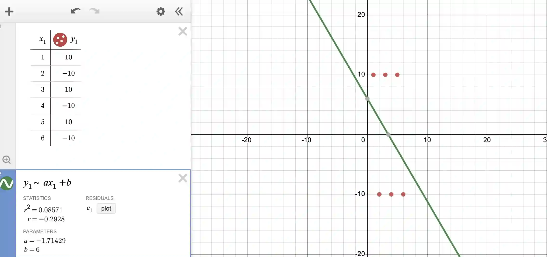
The r^2 value is 0.08, suggesting that the fit is really poor (as we can see on the plot when the fit is overlaid on the data points).

So what is the moral of the story? Make sure your data is suitable to be modeled as a line of best fit before embarking on the fitting exercise!

If you liked this blogpost and would like more experience with Desmos, learn how to make a heart shape with Desmos and other geometric designs.

If you enjoyed this blogpost, learn about math quadrants next! Explore Kodeclik’s Math courses and bootcamps! For more math fun, checkout our blog post on generating random numbers and on 100+ middle school math games.